
As AI adoption increases, so does the potential for model bias, defined as systematic and repeatable error in the predictions from AI systems that create unfair or prejudiced outcomes. In 2018, Gartner predicted that “85 percent of AI projects will deliver erroneous outcomes due to bias in data, algorithms or the teams responsible for managing them.” Addressing this challenge is particularly critical for organizations because biased AI models may lead to discriminatory outcomes, draw regulatory scrutiny and cause major reputational damages.
This can happen when the dataset used to train an algorithm reflects real-world inequalities between different demographics, such as criminal records in the United States. When AI models are trained on biased data, they are more likely to perpetuate and even amplify existing biases, leading to unfair outcomes for specific demographics.
When AI models are trained on biased data, they are more likely to perpetuate and even amplify existing biases.
The GRADE algorithm that was used for university admissions is a good example of how existing bias can be amplified by machine learning models. The model was trained on prior admissions data to determine which applications constituted a “good fit.” However, once the model was put into production, it simply overfits prior admissions decisions rather than actually assessing candidate quality. If these decisions had been used in practice, it would have amplified existing biases from admissions officers.
Despite best intentions, bias can creep into a machine learning model in a variety of different ways.

Exposure to protected features and their proxies
One of the most common, yet avoidable, ways models can become biased is through exposure to protected features. Yet, even if the model does not have access to protected attributes, they can still be learned through proxy features. Proxy Bias occurs when another feature fed into the model is highly correlated with a hidden, protected attribute. For instance, early predictive policing algorithms did not have access to racial data when making predictions but the models relied heavily on geographic data (e.g. zip code), which is correlated with race. Another example making the rounds on late night comedy, is this algorithmic hiring tool, that favored people with the name Jared that played high school lacrosse – attributes strongly correlated with race.
Biased Labels
Second, bias can emerge during data labeling in a few ways. The first is through Selective Labels. For instance, a college only obtains data on a student’s academic performance in college if an admissions officer chooses to accept the student, a bank can only obtain a borrower’s creditworthiness if a loan officer chooses to grant the borrower a loan, and police can only obtain data on whether a pedestrian is carrying contraband if they choose to search the pedestrian.
Labels can also be biased when they are collected from real outcomes suffering from taste-based discrimination. Taste-based Discrimination is a phenomenon where individuals discriminate even if there is no behavioral uncertainty. For example, an employer who needs to make a hiring decision and is faced with two employees, one from the majority group and one from a minority group, who have the exact same qualifications. If the employer would still choose to hire the first candidate, then this means they have a taste to do so.
The bias of the model depends on the form of the bias and the training of the model itself.
In some cases where both selective labeling and taste-based discrimination occur, and the decision-maker has access to unobserved data this can lead to Bias Reversal in an algorithm trained on that data. Bias reversal is a situation where the group that is discriminated against in the training data is subsequently favored by an algorithm or model trained on that dataset.
To understand the intuition behind cases of bias reversal, consider a scenario where police officers choose to search individuals for contraband based on the likelihood of their carrying contraband using both observed factors (time of the stop, demographic variables) and unobserved ones (such as the behavior of the individual). In the extreme case where police officers are so biased that they search all African Americans, regardless of underlying risk, then there will be no selection on unobservable behavior for African Americans in the training data. Thus, the more biased are police officers, the more favorable is the training data for African Americans, and hence the more the algorithm learns to favor African Americans.
This does not imply that biased data can never produce biased models, rather that the bias of the model depends on the form of the bias and the training of the model itself.

Representation Bias
Representation Bias occurs when the model predictions favor one subgroup of a population, better represented in the training data, because there is less uncertainty to their predictions. Amazon encountered this bias when building a facial recognition system trained on mostly white faces and drugmakers encountered this bias when the FDA excluded women of “childbearing potential” from clinical trials. The city of Boston also suffered from this issue, attempting to collect smartphone data from drivers going over potholes in an effort to fix road issues faster. In doing so, they involuntarily excluded elderly and underprivileged residents who are less likely to own smartphones.
If the disfavored subgroup is representative, this bias can often be addressed simply by rebalancing the dataset. However, if the disfavored subgroup is excluded altogether, addressing representation bias is much more challenging.

Measurement Bias
It is not just the training data and ground truth labels of a dataset that can be biased; faulty data collection processes early in the model development lifecycle can also corrupt or bias data. This problem is known as Measurement Bias and is more likely to occur when a machine learning model is trained on data generated from complex data pipelines. As an example, Yelp allows restaurants to pay to promote their establishment on the Yelp platform, but this naturally affects how many people see advertisements for a given restaurant and thus who chooses to eat there. In this way, their reviews may be unfairly biased towards larger restaurants in higher-income neighborhoods because of a conflation between their restaurant review and recommendation pipelines.

How to Measure Model Bias
To measure the fairness of an algorithm, there are a variety of metrics that may be appropriate depending on the aim of data scientists and stakeholders and the regulatory environment they operate in. To better understand the taxonomy of fairness metrics, we first need to understand the range of worldviews for model fairness.
We’re All Equal (WAE) is one such worldview. WAE views fairness as equal distributions of outcomes for all groups. In this world view, labels often stem from systemic bias in the real world, and so accuracy does not necessitate fairness. When you are confident that your training data and labels are unbiased, it may be more appropriate to take the What You See Is What You Get (WYSIWYG) approach. In a college admissions setting, The WYSIWYG worldview assumes that observations (SAT score) reflect ability to complete the task (do well in school) and would consider these scores extremely predictive of success in college.
Falling under the WAE worldview, the Impact Ratio is the most prevalent, commonly used by researchers and regulators alike. The Impact Ratio compares the proportion of favorable outcomes between different groups of people, such as the proportion of loan approvals for different racial or ethnic groups. Put another way, the impact ratio is calculated as the ratio of the proportions in each class receiving a positive prediction by the model.
An impact ratio of one means that each group receives favorable outcomes at the same rate, while a ratio of less than one indicates that one group receives fewer favorable outcomes than another. A ratio greater or less than one indicates that one group receives more favorable outcomes than another.
The most common threshold for identifying adverse impact comes from the Four-Fifths Rule. Many federal agencies (the EEOC, Department Of Labor, Department of Justice, and the Civil Service Commission) adopted the Uniform Guidelines on Employee Selection Procedures in 1978, and have used the rule since adoption. The Four-Fifths rule states that if the selection rate for a certain group is less than 80 percent of that of the group with the highest selection rate, there is adverse impact on that group.
Under the WYSIWYG worldview, a perfectly accurate model is necessarily fair because it matches the labels/observations you have on hand. To measure bias in this scenario, however, the aggregate accuracy is not sufficient. The overall accuracy metric can mask deficiencies in performance for subsets. Measuring the Accuracy Difference between different groups can expose underperformance and open the opportunity for performance improvements. This is especially important to identify for protected segments of the population.
When is Model Bias Justified?
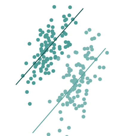
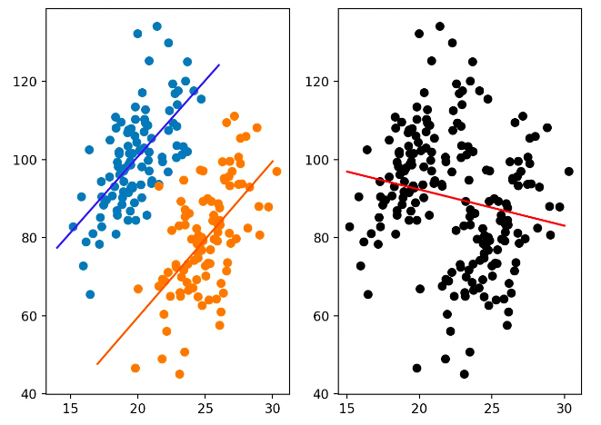
Often bias measured for a population is not preserved when examining subgroups, an effect known as Simpson’s Paradox. Simpson’s Paradox occurs when trends for partitions of a dataset differ from the trend in the dataset as a whole.
This paradox is shown in the illustration below. On the right side, a negative trend is displayed for the entire dataset, which could deceive the viewer into believing that the selected variables have a negative association. However partitioning the data into subgroups (shown on the left) illuminates the fact that the association is positive within each subgroup.
Berkeley admissions in the 1970s serve as an example of this phenomenon, when men were accepted at a greater rate than women overall. However upon closer examination of departmental subgroups, women had a higher rate of admission in most departments. The overall discrepancy stemmed from the fact that women had applied to departments with lower acceptance rates.
To determine when model bias is justified or unfair, one must determine the root causes of bias. If you are interested in this topic you should read, How to Measure and Debug Unfair Bias in ML. If the disparate impact arises from a model that does not rely on protected features or their proxies, the bias can be justified.
Try it yourself!
Get free, instant access to TruEra Diagnostics to de-bias your own ML systems. Sign up at: https://app.truera.net/
Learn More
Want to learn more about evaluating and mitigating bias on your own models? Join our community on Slack.