
Why does your ML model underperform? And how do you approach fixing it?
Improving the performance of a machine learning model is a huge challenge. ML models are fundamentally trained to optimize some performance or error metric– so why do models underperform, and how can we go about debugging this? In this post, we’ll provide an overview of the ways that a model’s accuracy may not meet the mark, and outline a framework to analyze and improve performance when it is not satisfactory. We’ll also use a few illustrative examples to demonstrate how the framework can be used in the real world.
Why is my model underperforming?
There are many reasons that a model can have poor performance when it comes to metrics like accuracy, but broadly, they can be grouped into six categories:
- Incorrect data and/or labels
- Insufficient data and/or labels
- Shifting data and/or labels
- An under or overfit model
- A model training procedure that is not aligned with the performance metric
- External bugs or pipeline changes
Let’s delve into each of these.
Data issues
The aphorism “garbage in, garbage out” is commonly used in ML. As many will say, a model is ultimately only as good as the data that it’s fed. There are a few ways in which data issues can manifest poor model performance.
Noisy data and/or labels: The most fundamental of data issues is that the data is simply wrong– perhaps the labels have been incorrectly assigned or a data collection pipeline is buggy. Incorrect data will necessarily lead to an inaccurate model. If, however, the incorrect data comprises only a small portion of the overall data this isn’t likely to be overly problematic. Common remedies of these problems include data cleaning and human input on label accuracy.
Insufficient data and/or labels: Perhaps the most common cause of performance degradation is that the training data simply isn’t sufficient to identify the true relationship between the inputs X and the outputs Y. Machine learning models are trained to capture the conditional relationship between inputs and outputs, or P(Y|X). However, there may be hidden features that are unobserved or difficult to measure and are therefore not in the X data that the model observes. For example, building a model that predicts the chance of rain would be hard without meteorological features. This can be remedied by adding more helpful features to X and/or expanding the precision of existing features.
In other cases, the data X may be insufficient to correctly learn P(Y|X) because certain segments of the population are not fully represented. For example, models often suffer to predict accurately on minority populations due to a dearth of training examples for these subgroups. Even if there are enough features to discern the actual P(Y|X) relationship, if the training points do not sufficiently cover the target concept, the actual P(Y|X) may be among several wildly different relationships that all accurately model the training data. This can be remediated by adding more training points on these low data regions where the model performs poorly.
Shifting data and/or labels: Shifting data is another common issue. This comes in two broad flavors: data drift and concept drift. Data drift, also referred to as covariate drift/shift, is a phenomenon where the input distribution P(X) has changed– for example, monetary features are subject to data drift due to inflation. A model that has learned P(Y|X) relies may only be performant on “known” inputs, so when P(X) shifts, it may not generalize well. Concept drift, on the other hand, is when the actual P(Y|X) relationship shifts itself– for example, the relationship between the number of bedrooms of a house and its selling price might shift over time also due to inflation. Changing P(Y|X) may necessitate retraining the model to capture the new relationship. Careful monitoring of data and labels can act as alerts of potential data or concept drift.
In addition, machine learning models are fundamentally attempting to model some behavior about the world, but that world is rarely static. External factors that modify behavior — such as inflation affecting consumer purchases, or a global pandemic changing traffic patterns — may also cause model performance degradation over time.
Model issues
Even once you’re sufficiently happy with the quality of your data, the way in which a model is trained and evaluated has vast implications on its performance. Here, we delve into two categories of low performance due to model issues.
Underfitting/Overfitting: Underfitting and overfitting are arguably the most famous and common of model issues. An underfit model is one that doesn’t accurately reflect the relationship between the inputs X and outputs Y of the training data even when such a relationship does exist. This may occur when a model is either under-parameterized and lacks the capacity to model P(Y|X), or even when the model hasn’t been trained long enough to learn this relationship, as is often the case with neural networks. Imagine training a neural network without a sufficient number of iterations of gradient descent — the model may not capture the nuances of the data.
In contrast, an overfit model relies too much on the nuances and noise of the training data. It then doesn’t generalize well to unseen data. If a model is overparameterized and/or fits itself to noise of the training data that is not representative of the real-world scenarios on which it will operate, it is indicative of overfitting. Careful analysis of a model’s performance on unseen data can expose overfitting.

Misaligned optimization and evaluation: An often overlooked model issue is that the chosen training procedure isn’t well-aligned with the performance metric that is used as a success criterion. That is, when training the model, we may be optimizing one metric but evaluating its final performance on another fairly different metric. For example, suppose we have a classifier that is trained to minimize log-loss on a dataset, but is evaluated using precision or recall– on imbalanced datasets, it’s unlikely the classifier would do well.
Pipeline issues: Machine learning models are not trained in a vacuum. In many settings, models rely on pipelines of engineered features that are aggregated from a variety of sources. As such, pipeline failures or code changes upstream of the model training or serving itself can have vast implications on model performance.
A framework to debug performance issues
Now that we have established the myriad reasons that a model can underperform on data, how do we go about addressing them? For the fastest, most effective outcomes, it is best to follow a systematic, four step approach: evaluate, narrow, analyze, and mitigate.
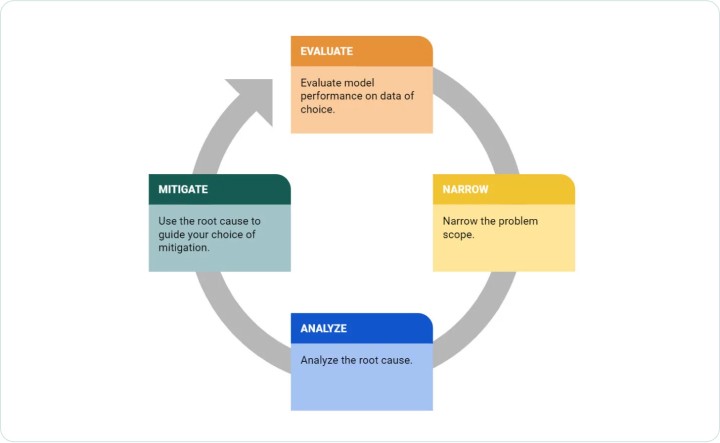
Figure 1. The 4 step framework for debugging ML model accuracy issues.
1. Evaluate model performance on relevant data.
Before even beginning to debug a performance issue, it is important to first clearly identify the population you are using for your analysis. Is the performance on the training data low? Is the performance on the test set low? Are you specifically debugging a performance drop between two different datasets? Each case will impact how you may approach debugging:
- If the model has low training accuracy, then either the model is unable to capture a relationship between inputs X and outputs Y, or such a relationship is not strong in the first place. If the former, the model may be underfit to the training data. Otherwise, the relationship P(Y|X) which the model is attempting to learn may be inherently noisy. Alternatively, you may not have sufficient data to capture the problem.
- If the model has low test accuracy, first check the accuracy of the model on the training set. If it is low, it is indicative of a problem during model training such as underfitting or inherent noise as described in the prior bullet point. Otherwise, high training accuracy with low test set accuracy is strongly indicative of overfitting. Regularization and other strategies to modify the training procedure of the model and decrease overfitting will help here.
- If the model has a drop in performance across different datasets, this is likely indicative of either overfitting or a change in the data/label distribution. If the inputs X or outputs Y have shifted over time, your model may not be able to generalize to these changes, and performance will degrade. Even more serious is when P(Y|X) itself has changed (concept drift) — in this case, the underlying relationship between inputs and outputs is not the same as it was when the model was trained, and the model may require retraining on newer data.
- If the model performs poorly on a segment of the population, contextualize the magnitude of the problem with the size of the segment. Is this a large segment that represents a sizable chunk of the population? Did the model perform well on this segment for the training or test datasets? Alternatively, if this is a smaller chunk of the population, did you have enough data to model the segment well originally?
- If you are attempting to debug single-point misclassifications or errors, it’s helpful to rely on a local explanation technology. Why did the model make its predictions for the given point? Do the features driving the prediction seem reasonable? It can help to zoom out: how is the model performing in the neighborhood around the point of interest?
2. Narrow the problem scope
Once you have identified the datasets where the model performs poorly, it then makes sense to narrow the problem scope. It would be difficult to come up with a targeted action plan if we treat the dataset as a single unit, since the model may not perform at a uniformly poor level on all of the points in the dataset. Instead, can we break down the problem by identifying specific regions of data where the model exhibits particularly poor performance? Are there any anomalous signals that correlate with the occurrence of the problem? This could be a data quality violation such as missing values, a change to the ground truth rate, shifting data values, a data processing pipeline bug, or even an external event that would catalyze a change.
3. Analyze the root cause of the problem
Next, try to find the root cause of the problem. Are the high error regions well represented in the training data? If not, then the problem may simply be because the model has not seen enough examples of this kind of data. If the problematic region is already well covered in the training set, then the low performance of the model may be indicative of other problems such as noisy labels. Also, identify if there is any data drift by examining how the distribution of each feature has changed, and see if the model’s performance suffers disproportionately more on points that look “newer” to the model. In addition, examine whether and how the label distribution has changed alongside any data shift — for example, has the proportion of points with a positive label suddenly changed? This may indicate concept drift in addition to or in place of solely data drift.
In addition, use explanation frameworks to better understand the model’s decision making. What features are driving model predictions? Do those features make conceptual sense and are they changing over time? Are there particular values for the important features that correlate with lower model performance, which may indicate that the model is overfitting or over-relying on ranges of that feature?
4. Attempt to mitigate the issue
Finally, use the root cause analysis to guide your choice of mitigation. Let’s walk through a few potential insights from root cause analysis along with amelioration strategies:
- If a particular feature or set of feature(s) strongly contributed to the low performance, you may choose to remove or regularize the feature so the model doesn’t overfit on noisy feature values. Keep in mind, however, that the most important features within your model may naturally contribute to error as the model is relying on them to make its prediction, which can sometimes be wrong. Thus, compare how the feature contributes to error against its overall influence on model predictions.
- If there is data or concept drift, your model likely needs retraining. Add data or labels that are representative of the shift to your original training data, or consider adding alternative data sources that would better capture the factors that led to features drifting.
- If there are noisy labels that don’t match with the labels of similar points, you may have mislabelling errors in your dataset. Identify these points and bring a human in the loop to sanity check labels.
By choosing a mitigation strategy that is guided by root cause analysis, model developers can be more targeted when debugging and improving models.
The framework in practice
Here, we’ll walk through an illustrative example to demonstrate how we can apply the performance debugging framework to understand and fix model performance issues.
Situation: determining home loan credit worthiness
Imagine the following scenario: you are tasked with training a binary classifier to predict the credit worthiness of individuals applying for home loans. You are given some historical dataset to train and evaluate your model, so you first split the available data into training and validation sets. Next, you experiment with various model architectures by training a number of different models: a logistic regression model, a random forest, a gradient-boosted tree ensemble (GBM), and a support vector machine (SVM). You then observe the following classification accuracies on the train and validation sets, Figure 2.
First analysis – Classification accuracies on various model types
| Dataset | SVM | GBM | Logistic Regression | Random Forest |
| train | 70.06% | 71.54% | 65.34% | 79.45% |
| validation | 67.01% | 71.10% | 65.47% | 70.33% |
Figure 2. The first pass at analyzing the accuracy of the model demonstrates underfitting in logistic regression and overfitting in random forest. Image by author.
You see that the logistic regression model underfits to the data while the random forest heavily overfits. Thus, you pick the gbm (gradient-boosted tree model) as it appears to do best on the validation set. But how do you ensure that your model will perform well in production? Let’s apply the performance debugging framework.
1. Evaluate model performance on various data
First you want to evaluate how this model will perform with data that is as close to a “real-world” scenario as possible. You work with the data team to get some real examples of the production data. Then you run your model on this data and observe the following result, as shown in Figure 3.
Second analysis – Testing with new “real-world” data
| Dataset | Classification Accuracy |
| test | 67.60% |
| validation | 71.10% |
Figure 3. After testing the model with a new set of data to approximate real world conditions, the model’s accuracy is lower. Image by author.
The model performs quite a bit worse on the test data! Now what?
2. Narrow the problem scope
Let’s narrow down the problem. The test data contains points with very different characteristics. It can be hard to formulate targeted plans to address this performance issue if we’re using the whole dataset as a logical group for which we’re trying to optimize. Even if a model has low overall accuracy on a dataset, it may not necessarily be uniform– the model may perform well on some pockets of points and much worse than average on others. So instead of thinking of a dataset as a monolith, it is often better to narrow the problem by finding high-error regions within the dataset. We can then focus on trying to understand the root cause behind the poor model performance in each of these regions and formulate a plan to mitigate the issue.
How do we identify these features or segments? One way is to isolate high-error features; that is, computing how much each feature contributed on average to the model error for each split (for example by using QII), and seeing which features shifted the most in their contribution between two splits (train and validation).
For example, are the top 5 features that contributed to the drop in performance, as seen in Figure 4, following.
Analyzing the features contributing to model error shift
| Feature | Contribution to Model Error Shift |
| NumSatisfactoryTrades | 28.34% |
| ExternalRiskEstimate | 19.62% |
| NetFractionRevolvingBurden | 10.32% |
| PercentInstallTrades | 7.60% |
| MSinceMostRecentDelq | 5.74% |
Figure 4. After isolating high-error features, we can see that two features contribute most significantly to model error shift. Image by author.
NumSatisfactoryTrades and ExternalRiskEstimate contributed to almost half of the instability! Let’s go even deeper. What specific feature values of NumSatisfactoryTrades and ExternalRiskEstimate are problematic? Let’s run an exhaustive search on continuous ranges of values for these features and see which segments significantly contributed to the low accuracy. In other words, we want a slice of the problematic feature that has low accuracy and yet is fairly sizable.
Looking at the NumSatisfactoryTrade feature, we find that the three most problematic slices are as follows in Figure 5.
Drilling down into the feature NumSatisfactoryTrade
| Segment | Accuracy | % of population |
| 11.0 ≤ NumSatisfactoryTrade ≤ 15.0 | 53.93% | 17.8% |
| 12.0 ≤ NumSatisfactoryTrade ≤ 15.0 | 54.16% | 14.4% |
| 0 ≤ NumSatisfactoryTrade ≤ 9.0 | 40.00% | 6.0% |
Figure 5. Model performance is less accurate when this feature is in the 11.0 to 15.0 range, impacting over 17% of the population. Image by author.
When the NumSatisfactoryTrades is in the 11.0-15.0 range, the model performs fairly inaccurately on a sizable chunk of the population.
Similarly, for the ExternalRiskEstimate feature we find the three most problematic slices:
Drilling down into the feature ExternalRiskEstimate
| Segment | Accuracy | % population |
| 71.0 ≤ ExternalRiskEstimate ≤ 75.0 | 50.75% | 13.4% |
| 71.0 ≤ ExternalRiskEstimate ≤ 77.0 | 55.56% | 18.0% |
| 72.0 ≤ ExternalRiskEstimate ≤ 75.0 | 48.15% | 10.8% |
Figure 6. Model performance is less accurate when this feature is in the 71.0 to 5.0 range, impacting over 13% of the population. Image by author.
The problematic segments here are fairly compact as well. Picking one, the 71.0-75.0 range seems quite problematic and sizable.
To improve the performance on these problematic regions we should understand the cause of the issue. Why does the model perform poorly on these segments?
3. Analyze the root cause of the problem
One common reason for poor performance in a region is that the training data lacks many points in that area– as a result, the model either neglects that region during training or overfits to it. To debug this, let’s see how well represented these segments are in the training set.
Identifying segment representation in a training set
| All | 11 ≤ NumSatisfactoryTrades ≤ 15 | 71 ≤ ExternalRiskEstimate ≤ 75 | |
| Accuracy (test) | 67.6% | 53.93% | 50.75% |
| % of population (train) | 100% | 16.62% | 1.65% |
| % of population (test) | 100% | 17.80% | 13.40% |
Figure 7. ExternalRiskEstimate is under-represented in the training set, at only 1.65%, versus 13.40% in the test set. Image by author.
It seems that the ExternalRiskEstimate segment is vastly under-represented in the training set compared to the test set! This explains this feature’s effect on the accuracy degradation.
The problematic NumSatisfactoryTrades segment however, is well represented and so further investigation is necessary. However, upon manual inspection, we find that the segment in question has several training points that might be mislabelled. This is further corroborated by the fact that several other robust models we train view these potential mislabelled points as anomalous. Consulting with domain experts, it looks like the data gathering process has failed and the labels on these points have been erroneously flipped!
4. Attempt to mitigate the issue
We’ve determined a set of initial hypotheses on why the model is performing poorly on these high error segments, so next, let’s formulate a targeted plan on how to address each of these issues.
Let’s focus on the 71 ≤ ExternalRiskEstimate ≤ 75 segment first. The problem with this segment is that it is severely under-represented in the training set. So then we work with the data team to collect additional data, targeting the 71 ≤ ExternalRiskEstimate ≤ 75 segment and retrain the model. Here’s the performance of the latest model, in Figure 8.
Impact on model accuracy of additional data for ExternalRiskEstimate
| All | 71 ≤ ExternalRiskEstimate ≤ 75 | |
| Accuracy (test) [model v1] | 67.6% | 50.75% |
| Accuracy (test) [model v2] | 70.8% | 62.69% |
Figure 8. The accuracy of Model V2 is improved when additional data is collected for this specific range for ExternalRiskEstimate. Image by author.
A significant accuracy gain on that segment, which is reflected on the overall accuracy bump on the test set!
Now let’s move on to the next high error segment (11 ≤ NumSatisfactoryTrades ≤ 15). During the root cause analysis step we found that the points in that region have been mislabelled. Simply correcting the labels for these points and retraining gives us the following model performances, as seen in Figure 9.
Impact on model accuracy of correcting data labels for NumSatisfactoryTrades
| All | 11 ≤ NumSatisfactoryTrades ≤ 15 | |
| Accuracy (test) [model v2] | 70.8% | 61.79% |
| Accuracy (test) [model v3] | 73.2% | 75.28% |
Figure 9. The accuracy of Model V3 is improved when data labels are corrected for this specific range for NumSatisfactoryTrades. Image by author.
Again we see a significant accuracy gain on that segment! Now the accuracy of that segment is comparable to the whole population.
In summary
Building high-performing machine learning models can be challenging– especially when you see a low accuracy or AUC without any clear path to improvement. However, by breaking down the core reasons for why a model may be underperforming, and by using a methodical approach to debug performance issues, model developers and data scientists can more quickly debug and improve their models.
Authors:
Divya Gopinath
David Kurokawa
Arridhana Ciptadi
Anupam Datta