
From recommendation engines in retail to credit risk classifiers in finance, machine learning (ML) models have become a vital part of many industries. As ML models adoption increases it is essential for data scientists to provide explanations for their model’s decisions to business stakeholders.
One way to explain a model’s behavior is to use feature importance , which measures the marginal contribution of each feature to a model’s decisions. In practice, it indicates how many records are strongly affected by a feature.
In this blog post, we first discuss how to interpret feature importance, then, how to use feature importance in explaining and debugging ML models, and finally how to best calculate Shapley values, a popular metric for calculating feature importance.
How to interpret feature importance?
Feature importance is calculated by taking the average of the absolute value of a given feature’s influences over a set of records. Consider a classification model trained to predict whether an applicant will default on a loan. This model might use features such as income, gender, age, etc. Let’s consider the importance of the “income” feature to the model’s decisions. If the importance of income is 0, this implies that for any record, the influence of income is the same for this feature (i.e. it always contributes X to the model score). So even if an applicant changes their income, the model will not react and will simply do the same thing. We may then say that the applicant’s income is “not important” and can be replaced with a constant. In contrast, if the feature’s influence on the model output changes as the applicant’s income varies, this metric will increase. The more impact that income has on the model’s behavior, the more important it is.
Now that we understand feature importance, we turn to feature influence. There are different frameworks for calculating influence, such as LIME, Integrated Gradients, and Shapley Values. Choosing a framework for calculating feature influence depends on multiple factors, but here we focus on Shapley values, which was originally introduced in game theory. The key idea is that these features (“players”) make marginal contributions that drive the model’s decision “game” towards its final outcome.Shapley values are highly appealing in machine learning because they satisfy specific axioms ensuring that they reflect a model’s decisioning process. Also, they only require access to a model’s inputs and outputs, allowing us to explain “black box” models. However, Shapley values have some practical shortcomings when it comes to their calculation.
Using feature importance to improve ML models
Feature importance is a powerful tool in a data scientist’s toolkit. Data scientists can use feature importance to perform various tasks, such as feature selection and feature engineering, in a highly principled and interpretable way.
Indeed, when we perform feature selection, we are deciding which features to keep as inputs to the model. A typical workflow might involve trial-and-error, i.e. dropping a feature (group), training a model, evaluating accuracy, and repeating. In a more directed workflow, we can decide to drop features that have low importance, as these features are known to have a small impact on the model’s decisions. Dropping these features can even improve a model as these features can add spurious contributions to the original model.
Further, computing feature importances is useful when performing feature engineering, i.e. combining or rescaling features to improve model performance. We can calculate the importance of engineered features to determine whether they are impacting the model’s decisions or not.
In addition to conventional workflows, visualizing feature influences allow us to assess the conceptual soundness of models. The idea behind conceptual soundness is that changing certain features should have a sensible effect on the model’s output. Here is an illustration,, consider the influence sensitivity plot (ISP) for the median income (“MedInc”) feature of the California housing dataset, which shows the median income of residents in the house’s neighborhood. An ISP is a scatter plot for a single feature showing the feature’s influence (y-axis) against its value (x-axis) for each record (read here for more on ISPs). A higher influence value means that the model’s decision on the point is driving the model towards a more “positive” outcome (in this case, a larger dollar value).
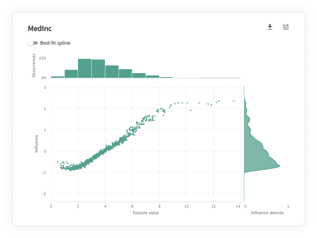
To evaluate conceptual soundness, look at the ISP and ask yourself : “As we increase MedInc, what should happen to the model’s predictions?” If you’ve been thinking about purchasing real estate, then you might intuit that houses in a neighborhood with higher MedInc will be more expensive. The ISP supports this intuition, as higher MedInc values result in higher influences, and we may conclude that our model is conceptually sound.
Calculating Shapley values
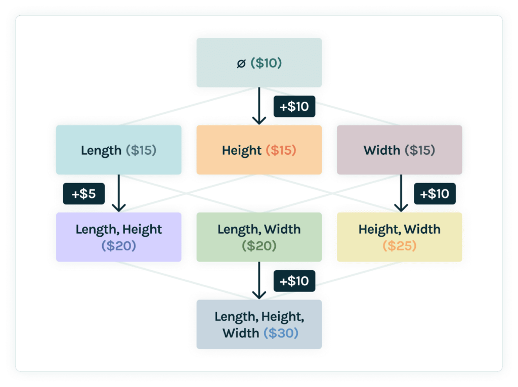
Now that we know how to use feature importances, let’s discuss how to calculate Shapley values. One popular open-source library for calculating Shapley values is SHapley Additive exPlanations (SHAP). The basic idea behind SHAP is to calculate the marginal contribution of a feature when the feature is added to a model that does not contain the feature. For example, the figure below represents a model predicting the price of a coffee table using “Height,” “Width,” and “Length.” Each node is a version of the model that uses the stated feature(s), where the root model simply uses the mean value of the training dataset. SHAP finds the influence of “Height” by taking a weighted sum of the marginal contributions by “Height” (highlighted in orange in the Figure).
In practice, SHAP relies on taking the expected value over several different values of the added feature (“Height” in the above example), which can be computationally costly. However, the original SHAP paper details optimizations for different types of models, and these model-specific implementations are available in the SHAP repository. In addition to SHAP, the Quantitative Input Influence (QII) algorithm provides an even more efficient method for calculating Shapley values.
If you want to use SHAP or QII to help explain your ML models, then click here to get free access to TruEra Diagnostics! For readers already using SHAP, you can go beyond explainability with TruSHAP, a lightweight SHAP extension that lets you analyze your models in TruEra with no additional lines of code.