
In a previous article, we analyzed a model for predicting Airbnb listing prices in San Francisco. The model was an XGBoost model trained on Airbnb data scraped by Inside Airbnb and hosted by OpenDataSoft. In this article, we’ll take a step further into the model’s performance in other cities. Transfer learning can be a useful part of your workflow for classical machine learning – not just deep learning tasks! Targeted mitigation of the true cause of drift in new contexts can improve the general performance of machine learning models.
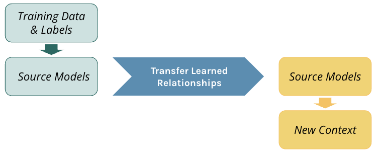
Transfer learning seeks to leverage feature representations from a pre-trained model and leverage them either to make predictions or to help train a new model on a new task. In this example, both the source and new context for our model share the same feature space, yet the mapping of features to the target differ.
Drift across Contexts: Taking a San Francisco-trained model to Seattle
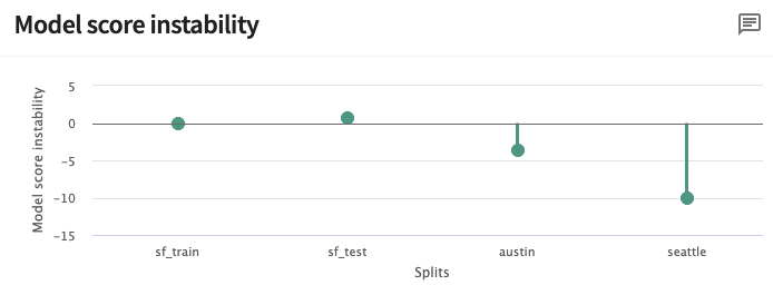
Examining the model score instability of the San Francisco trained model, the model is relatively stable with a difference of means near zero for both of the San Francisco data splits (sf_train, sf_test). Austin and Seattle tell a different story with nonzero model score instability (shown below). The mean score in Seattle is approximately ten points less than in San Francisco, more unstable than Austin. Because of that, Seattle will be the primary data split for examining the true cause of drift.
Finding the True Cause of Drift
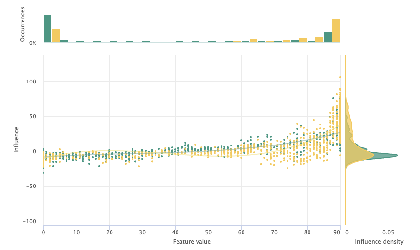
The first features to examine are availability. These features contain each listing’s available nights over a given time period, shown as a suffix (e.g. _365). In combination, these features are the largest contributor to error drift. Availability_90 (11.86%) and availability_365 (9.98%) are particularly egregious contributors to error drift. Shown on the x-axis of the Influence Sensitivity Plot (ISP) below, there is a large distributional shift between San Francisco and Seattle for extremely low and extremely high availability. We can also see this shift in the influence density, shown on the y-axis. Seattle (yellow) has a higher density of positive feature influence, while San Francisco (green) has a much larger spike in influence slightly below zero. Note: we’re not assigning causality to the real world, we are observing how each feature contributes to the model’s score.
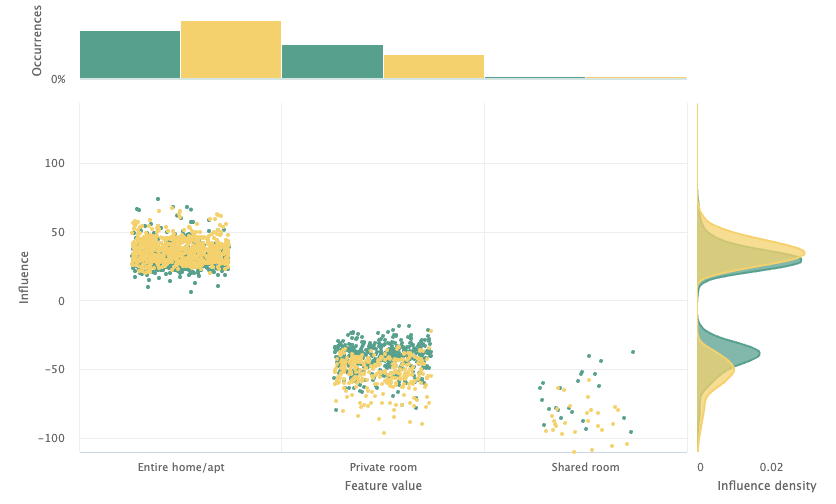
Room type is another feature that heavily contributes to error drift in Seattle. Examining its influence sensitivity plot, there is a divergence in the feature influence for private rooms. Private rooms have a more negative average influence on the model score in Seattle compared to San Francisco. While both availability and room type are large contributors to error drift, this drift is not due to issues with the features. Instead, they are symptoms of transferring the model from San Francisco to a new context. We should keep looking…
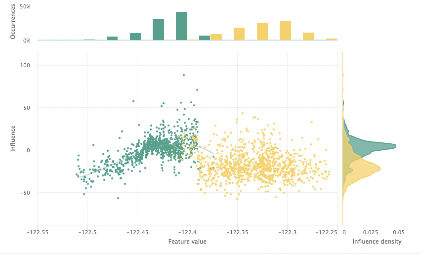
Latitude and longitude tell a different story, contributing 10.27% and -6.72% to error drift respectively. It is intuitive to understand why these features may not be general, as the model learned relationships between locations in San Francisco and the listing price that are not applicable. The grouped ISP of latitude comparing the San Francisco test data and Seattle is shown below for illustration. To make latitude and longitude more effective general features, we can transform them by target encoding.
Target Encoding: Using latitude and longitude to make the model more generalizable
The learnings from San Francisco locations do not translate to other cities, contributing substantially to the error drift of the Seattle data split. Rather than just removing the features all together, we can perform a more targeted mitigation by transforming these feature values to have more shared value distribution. One way to do this is target encoding. Target encoding is the process of replacing each categorical feature value with its target variable average. You might say – latitude and longitude are not categorical variables! This is true – before we can target encode these features, we’ll first transform them to their quintile values. Once we’ve transformed the values to quintiles, we can then replace latitude and longitude quintiles with their average listing price. The target encoder used is shown below.
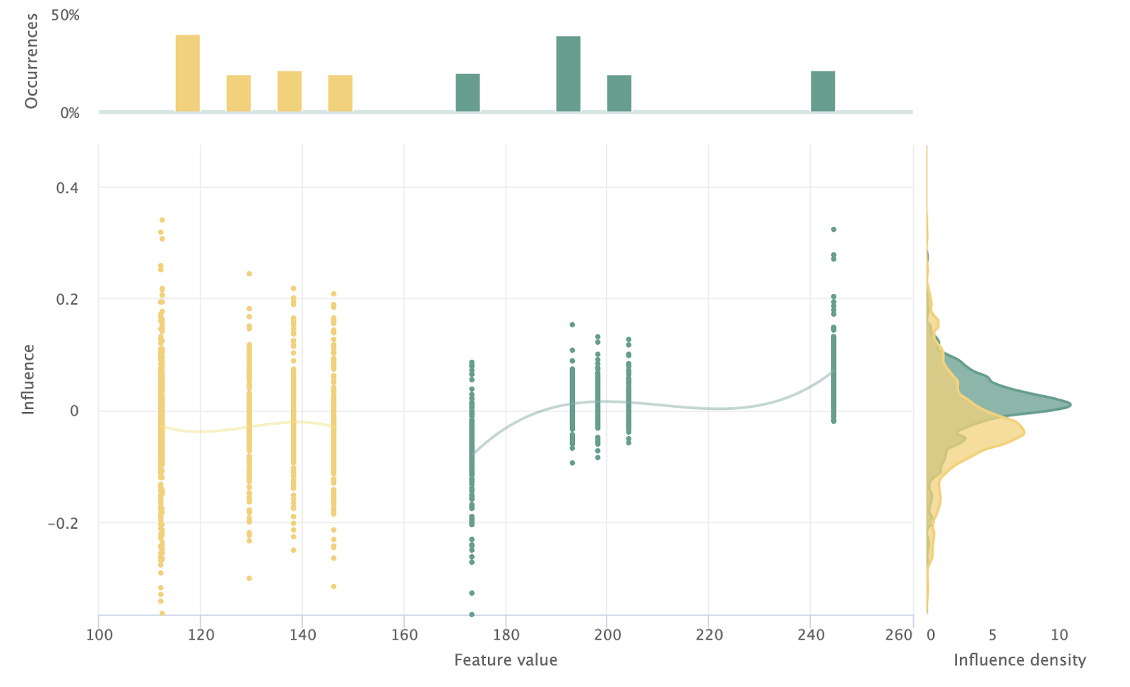
By making this change, we drastically reduce the gap of mean absolute error (MAE) between the San Francisco train and test sets from $38 to $12. After making this change, it became clear that the difference in listing prices was the true cause of drift. San Francisco’s average listing price of $200 compared to Seattle’s $120 leads the model to systematically overestimate prices in Seattle. The influence sensitivity plot for target-encoded Latitude clearly shows this lack of shared distribution. There is no overlap in average listing price between even the top quintile in Seattle and bottom in San Francisco. This lack of shared feature values makes the model unable to transfer knowledge of San Francisco’s target encodings to Seattle’s.
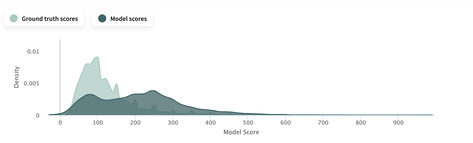
The model scores (dark) spread across a much higher range of prices than the ground truth scores (light green) also reflect this reality. Because our model is trained in only one city, it has no chance to pick up on this difference in average listing price between cities. If we hope to build a reasonably accurate general model, we must adjust.
With this discovery, there are a few possible mitigation strategies. The first is that we can increase the granularity of our target encodings, perhaps in two dimensions as a grid. More granular encodings would allow for an increased potential for overlap – what we need for transfer learning. The second is to change the task in a way that creates more overlapping distribution for the target.
Let’s first try the more granular approach to target encoding. Instead of using one-dimensional quintiles we will instead create a 5×5 grid over San Francisco and encode the average listing price for each grid, shown below.
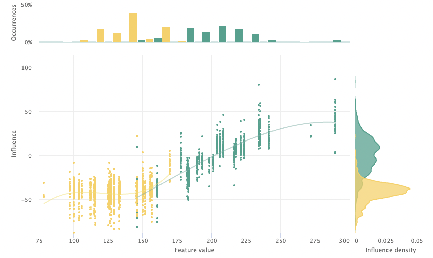
Using this new approach there is now overlap between the encodings of the two cities, enabling successful transfer across them.
Applying the Model to Austin, Texas
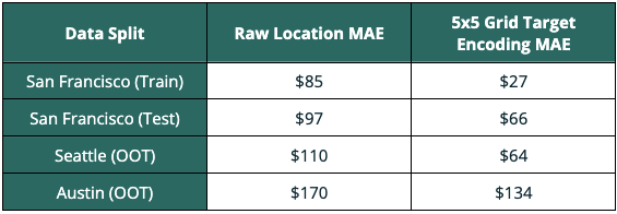
Now that we’ve made this change, we want to take a second look at the Austin data split. This change dramatically improves our model’s performance across all data splits. Below you can see substantial mean absolute error improvement in Seattle Austin – indicating that our drift mitigation strategy was successful.
Reframing the Prediction Task to Improve MAE
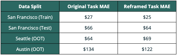
To further compensate for this inherent difference in market conditions across cities, we will also try our second targeted drift mitigation strategy. By reframing the task our model is learning, we can transform the target variable to a range that is shared across all cities. Instead of listing price – we will instead predict each listing’s standard deviations from the average listing price. In practice, the mean and standard deviation of listing price could then be easily discovered in new cities and applied to calculate the predicted actual price. Below the data and labels are extracted from TruEra before being transformed to their standard deviations from the mean. After transformation, the model is retrained using the extracted training data and transformed labels. Last, the retrained model along with each data split are then added to a new data collection.
By reframing the task, the model’s performance showed moderate improvement in Austin and slightly diminished in Seattle. While this mitigation strategy was not as fruitful as the first, the resulting performance improvement indicates a small success.
Targeted Mitigation of Transfer Learning Drift
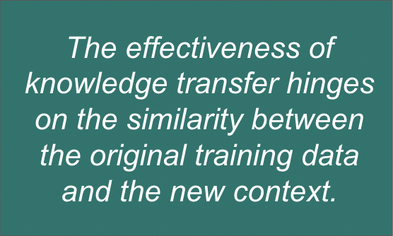
In this experiment, investigation into the drift of our San Francisco-trained model allowed the discovery of its true cause. From the true cause, targeted mitigation strategies yielded a more generally performant model. While retraining smaller models to mitigate drift has low cost, doing so can often hide the true cause. By finding the true cause of the drift, we found large performance improvements through two-dimensional target encoding. Additional improvement in the most dissimilar context (Austin) was found through reframing the prediction task to a more general one. However, performance in Austin significantly lagged that of Seattle – a direct result of its larger difference from the training data.
Through debugging a model’s drift in a new context, we were able to craft a new champion generalized model. Even so, the idiosyncratic value of big houses and air conditioning in Texas can only be learned on location…
Try it yourself!
Get free, instant access to TruEra Diagnostics to debug drift for your own model. Sign up at: https://app.truera.net/
Learn More!
If you’re interested in learning more about how to explain, debug and improve the quality of your ML models, join the community!