
This article was co-written by Arri Ciptadi.
Motivation
In the United States since 2000, an average of 70,072 wildfires burned an average of seven million acres per year. This rate doubles the average annual acreage burned in the 1990s (3.3 million acres). In just 2021, nearly 6,000 structures burned, sixty percent of which were residential. If wildfires could be predicted in advance, those predictions could aid in targeted mitigation efforts, reducing the likelihood and overall impact of these fires. As a company with a headquarters in California, wildfires and their impacts are of strong interest to our team.
Testing in a High Stakes Environment
Using high resolution data, we will predict the likelihood of fire in any given month and location in the western United States. As the frequency and severity of fires increases over time, the stakes for accurate prediction of wildfires are high and only getting higher. An environment with high stakes such as this mandates high quality for any ML system deployed. To do so, we will establish performance thresholds prior to model training, and then increase these thresholds iteratively as our model improves its performance.
This proactive testing and performance evaluation approach is uncommon today in machine learning. Relatively early on in its maturity curve, machine learning has yet to graduate into systematic testing like software testing did in the 1990s. Unlike software, which throws exceptions, machine learning models often fail silently. As a result, data scientists who start model development without a testing plan often run into performance problems and model development takes longer than if a testing plan is part of the process from the outset. Rigorous model testing can debug learned issues and improve robustness when deployed into production.
Constructing the Data
To tackle this prediction task, we accessed the Global Fire Emissions Database (GFED) to extract burning, emissions, and biosphere data. This data was available at the spatial resolution of 0.25 degrees on a monthly basis from 1997 onwards.
Below is a descriptive table of the data used:
Stored in HDF5 format, we used the h5py package to extract the data into a pandas DataFrame. The Hierarchical Data Format version 5 (HDF5), supports large, complex, and heterogeneous data using a “file directory” like structure. NSF NEON has additional information on the HDF5 file format.
Below, you can see how we accessed datasets stored in each HDF5 file using their keys. After extraction we flattened each dataset to create a Dataframe.
We format the modeling data with observations on the spatial dimension. Then, the features can be the burned fraction, emissions and biosphere data for each past month. The suffix of n minus the number of months back denotes the age of each feature.
Test-Guided Model Development
Before training the first model, we create performance tests with TruEra’s Test Harness. Performance thresholds can be established from domain knowledge, stakeholder requirements or an existing champion model. Establishing these thresholds prior to model training can then be used to benchmark new candidate models.
These tests will guide our iterative model development. To establish a target performance threshold, we consulted Predicting Forest Fire Using Remote Sensing Data And Machine Learning. In that paper, the authors use the FIRMS hotspot dataset with spatial granularity of 8x8km2 and a somewhat limited temporal dimension (only up to one year). The model, Agni, achieved AUC scores ranging from 0.80 to 0.85.
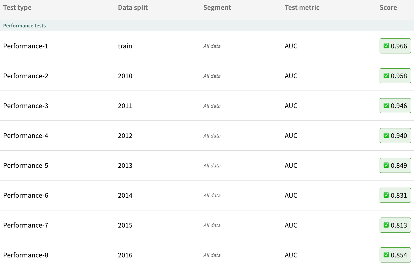
The baseline model will be tested against Agni’s performance. Thresholds established will warn if AUC falls below 0.85 and fail if AUC falls below 0.80. We train the model on data from 1997-2009 and test on data from 2010 onwards.
Baseline Performance
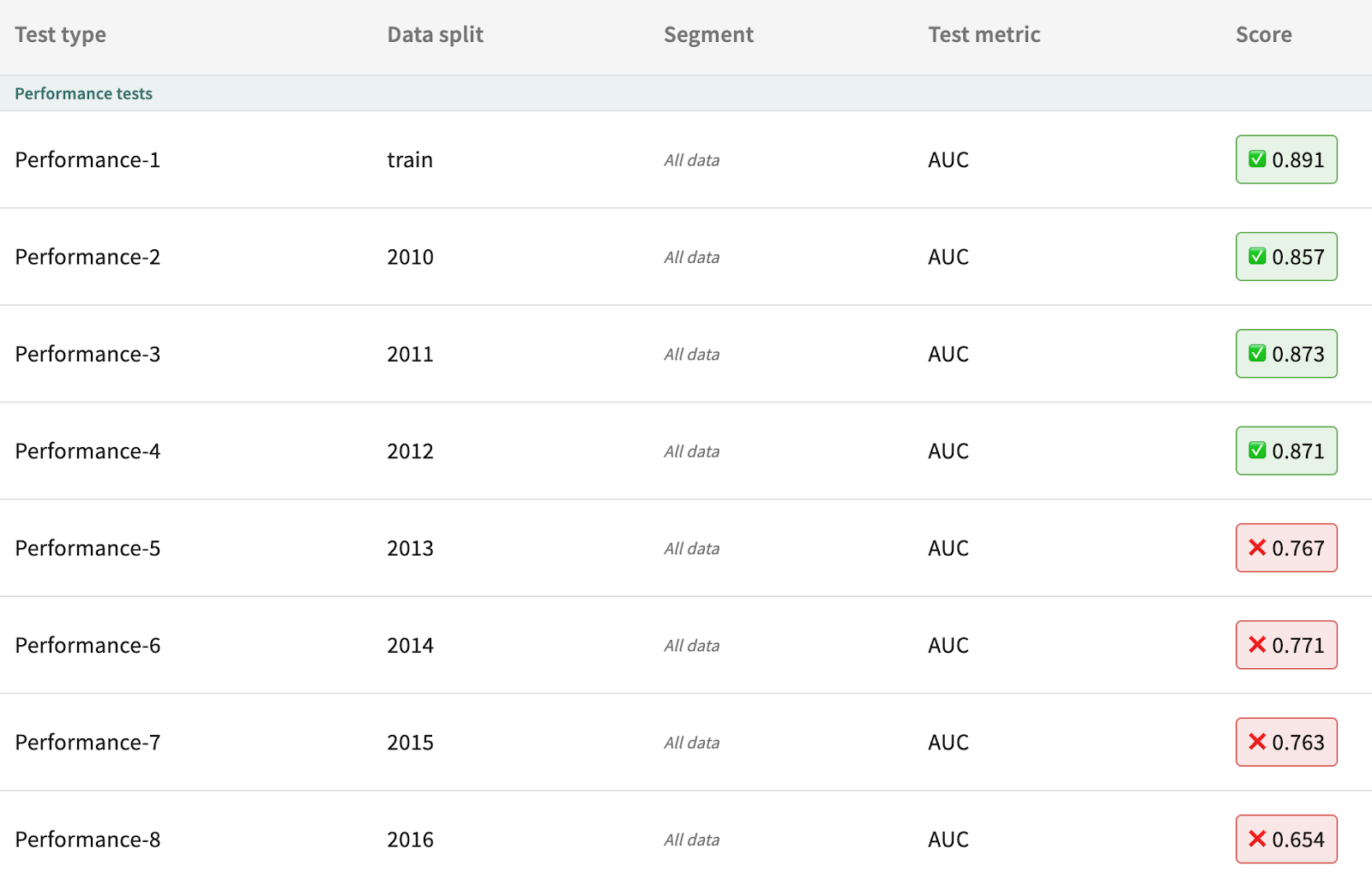
For this task we start with a linear model with a 2 year input window (i.e., to produce prediction for year x, the model will take as input data from year x-1 and x-2). Examining the tests, we can see this baseline performs poorly compared to the Agni-based testing regime. The baseline linear model passes zero performance tests, warning on 5 and failing 3.

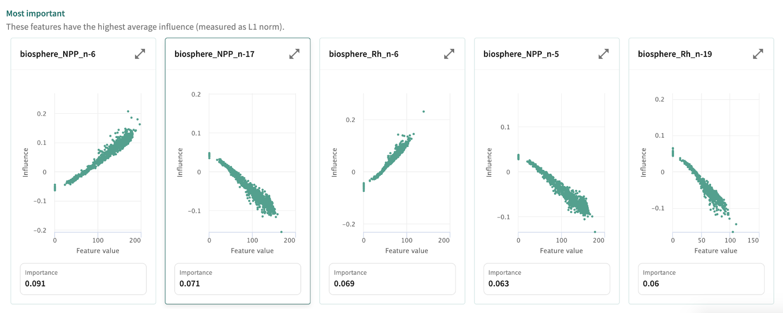
Examining the feature influence of this model, two of the top five features (biosphere_NPP_n-17, biosphere_Rh_n-19) are near the end of the input window. The features n-17 and n-19 correspond to data from 17 and 19 months from time of prediction respectively. This gives us a clue that we should extend the input window farther back into the past.
Extending the Feature History
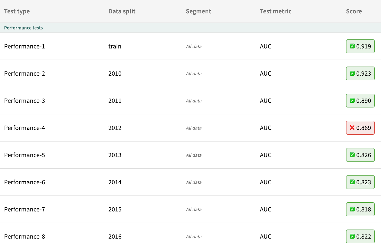
The literature around fire cycles broadly agrees that surface fire and torching potential is most likely in what’s called the gray phase (5 to 10 years following a fire). To account for this cycle, we will train another linear mode but with its input window set to ten years. After evaluation, we can see that the new linear model now passes 4 out of 8 performance tests.
From Linear to Gradient Boosting Classifier
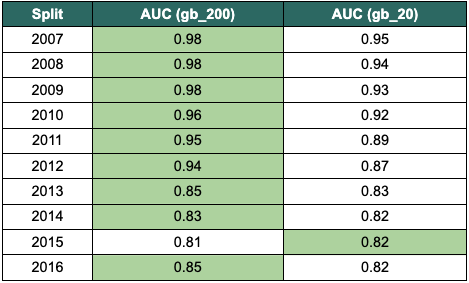
Now that baseline performance is established, we should update our testing scheme to fail relative to the linear model with an equivalent feature history window. To do so, we use the same add_performance_test() call and set fail_threshold_type to “RELATIVE” and add the reference_model_name argument. The code required to add this new performance testing scheme using the TruEra SDK is below.
From here, we will consider a more complex model: gradient boosting (GB) classifier. This GB classifier will have the n_estimators parameter (the number of boosting stages) set to 20. Using the new relative failure threshold, the GB model performs better on all data splits except for 2012. Shown by the absolute warning threshold of 0.80, the GB model meets or exceeds Agni’s minimum performance in all splits.
Increasing the n_estimators parameter to 200 further improves performance. Using both the warning condition against Agni and the failure condition relative to the linear model, gb_200 passes the performance tests for all data splits.
Selecting the Champion Model
At this stage, selecting the champion model is relatively easy. The gb_200 model passed all performance tests. For final verification, we will examine the two candidate models that meet Agni’s performance criteria in comparison to each other. Assessing the difference in AUC score, the gb_200 model outperforms the gb_20 model on all splits but one.
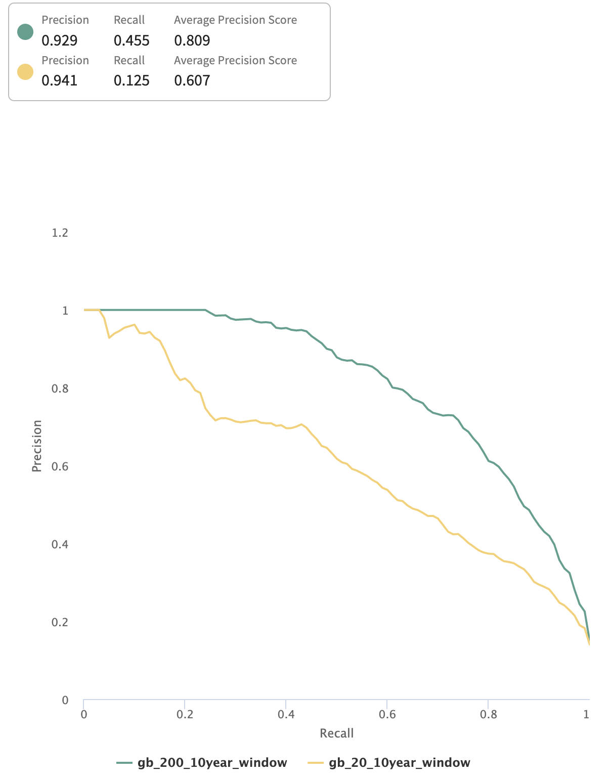
Comparing the precision-recall curves for the best performing split on each model, the gb_200 model takes a more convex shape. Its concave shape sustains substantially higher precision as the classification threshold is lowered, thereby increasing the recall of the model (correctly predicting more actual fires).
We can also visualize the champion model’s predicted fires (blue) to actual fires (orange) to see its performance. Notably, the model successfully predicted the fires along the southern coast of California from San Diego to Santa Barbara, the pocket of fires north of Sacramento, and the swath of fire extending from northeast Nevada, up through western Idaho to the southeast corner of Washington.
Automated Standard Testing for ML
In this blog we followed an iterative, test-driven approach to model development. We created a reasonably good model for predicting forest fires in the western region of the United States. Test-driven modeling helps to create a repeatable and standardized approach to building and assessing candidate models. Let’s hold our ML systems to a higher standard of quality, just like what’s expected for software.
Try it yourself!
Get free, instant access to TruEra Diagnostics to accelerate your model development. Sign up at: https://app.truera.net/
Learn More!
If you’re interested in learning more about how to test, explain, and debug your ML model – join the AI Quality Forum slack community.