We’ve written extensively on best practices for machine learning testing and debugging, to improve their performance, stability and fairness in production.
In this blog, we will walk through a practical topic: how to improve BQML model observability with TruEra.
TruEra’s SDK allows flexible ingestion of models, whether open source software (OSS) or proprietary. Our methods enable this via access to the model object, or only the data produced by a model. This flexibility simplifies integration efforts for model developers and platform owners.
The Challenge
Nowadays, software tools for creating and deploying machine learning models are a dime a dozen. Various MLOps frameworks have matured to support such models in production.
While the deployment & operations solutions have become more automated, with cloud service providers offering proprietary tools to help ML Engineers & MLOps personas scale & manage production ML pipelines, corresponding tools for data scientists to perform model testing & debugging have lagged behind: today, such tools are primarily code-first, and frequently, amount to use-case-specific, notebook-based templates. This lack of tooling maturity for data scientists makes it difficult to perform critical model-centric tasks prior to, and throughout, production deployment:
- Establishing correct tests & thresholds
- Performance debugging
- Analyzing overfitting
- Identifying consequential model drift
- Validating model fairness (when model predictions affect persons)
As a result, time is wasted maintaining code for custom model evaluation workflows. And visualization tools for these workflows often fall short of the interactivity and information density required to effectively analyze model behavior.
These challenges also create issues when attempting to communicate insights about models’ predictive behavior to stakeholders who are not code-first. Are there tools available to repeatedly capture key insights about your models’ predictive behaviors, and to communicate them clearly?
TruEra Diagnostics solves these problems. Let’s take a look at how you can easily register data generated during a modeling process to capture comprehensive analytics about your models’ predictive behaviors.
The Approach
Train a BQML model as normal
BQML has a wide variety of tools to create and use machine learning models. They offer various model types, data preprocessing, hyperparameter tuning, and weighting functions to accelerate a typically iterative, code-first approach to model development. Here, we will use a BQML tutorial dataset & model, with slight modifications, to demonstrate integration with TruEra Diagnostics.
Figure 1: Creating a boosted tree classifier using BQML
Note: the demo model is not performant. We will be able to easily observe why this is the case, within TruEra.
Generate Feature Attributions
Feature attributions are a core requirement for any platform that seeks to find the root cause of model quality issues, and we’ll need a way to generate them as part of this integration. TruEra enables flexibility for producing the feature attributions that power many of our debugging & explainability analytics. To integrate with your BQML pipeline, you have two options.
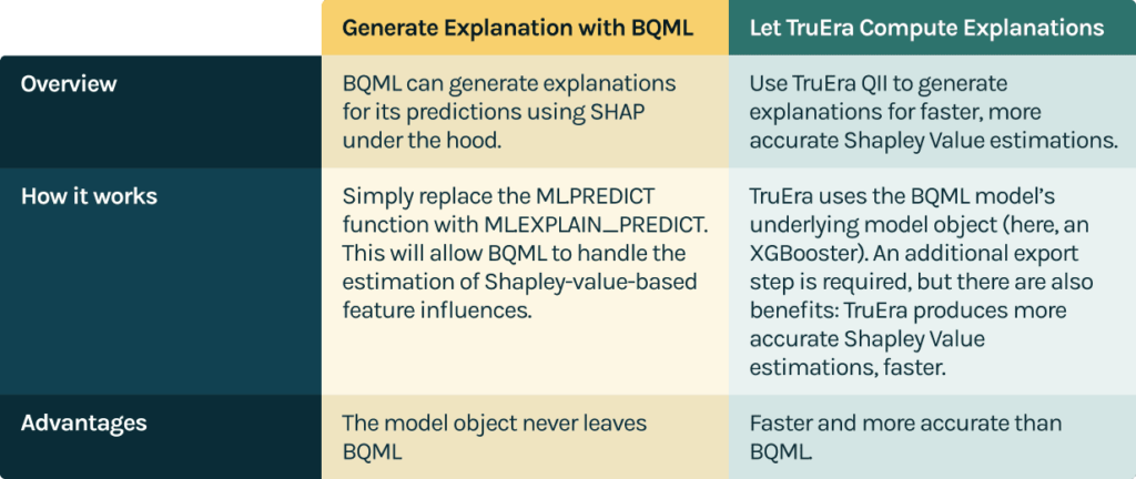
Option 1: Generate Explanations with BQML. Replace ML.PREDICT with ML.EXPLAIN_PREDICT, allowing BQML to handle the estimation of Shapley-value-based feature influences.
Option 2: Let TruEra Compute Explanations. TruEra uses the BQML model’s underlying model object (here, an XGBoost booster). An additional export step is required, but there are also benefits: TruEra produces more accurate Shapley value estimations, faster.
For the purposes of this demo, we will focus on option 1. But, option 2 is also straightforward: export the underlying booster from BQML, load it into a jupyter notebook, and generate predictions & feature influences using booster.predict() and tru.get_feature_influences().
Demonstration: BQML Model Registration in TruEra
In this example, we’ll use a notebook hosted in Vertex Workbench. But any Jupyter environment running Python >=3.7 will suffice.
Import TruEra. If you haven’t installed it yet, it’s available from pypi, or from the Resources page of your dedicated deployment. See TruEra’s Quickstart documentation for more details.
Authenticate & Create Workspace
Figure 3: Load the TruEra SDK & create a TruEra workspace
Set up BQ Client & poll data
Figure 4: Load the BigQuery python client to access your data
Note: depending on where you run this notebook from, you may need to use a service account key. You can find more information here.
Generating feature explanations using BQML
BQML lets users generate predictions & feature attributions with a simple query: ML.EXPLAIN_PREDICT.
ML.EXPLAIN_PREDICT generates feature attributions for all features in the BQML model schema, and also enables one to pass through additional columns from a table of interest (e.g., unique IDs, and labels, the latter of which are required to perform model performance evaluation).
Figure 5: Using ML.EXPLAIN_PREDICT to generate feature attributions
Note that the feature attributions are returned as an array of structs. We can unpack attributions/explanations using unnest commands.
Figure 6: Unnesting BQML-based feature attributions into desired formats
Now, we have our feature influences (feature attributions) in a format we can use: one column per feature, one attribution per row.
For demonstration purposes, we’ve combined the unnested attributions with the input data, the predictions, labels, and a unique ID column.
| visitid | os | is_mobile | pageviews | country | prediction_value | probability | label | pageviews_attr | country_attr | is_mobile_attr | os_attr | |
|---|---|---|---|---|---|---|---|---|---|---|---|---|
| 0 | 1482091790 | Android | True | 2 | United States | 3.896123 | 0.998879 | 0 | 1.955159 | -0.023513 | 0.030004 | 0.017490 |
| 1 | 1493475353 | iOS | True | 1 | Germany | 3.896123 | 0.998879 | 0 | 0.850784 | 0.183103 | 0.026549 | 0.018705 |
| 2 | 141638718 | Android | True | 1 | United States | 3.896123 | 0.998879 | 0 | 1.055159 | -0.023513 | 0.030004 | 0.017490 |
| 3 | 1474436567 | iOS | True | 7 | United States | 3.813677 | 0.998879 | 0 | 0.866688 | -0.032306 | 0.095131 | 0.671800 |
| 4 | 1473958029 | Linux | False | 6 | Panama | 3.797932 | 0.998636 | 0 | 0.469744 | 0.485413 | -0.006873 | 0.032664 |
Figure 7: BQML model input, output, and feature attribution data in ingestion-ready format
Note that ML.EXPLAIN_PREDICT provides predictions in both logits and probits/probability format. Here, we use logits, but either is supported. Depending on the model type and your use case, you may have reasons to use one, or the other, for evaluation purposes.
TruEra Project Configuration
Now, let’s ingest this data into TruEra. It only takes a few lines of code.
1. Project – Create a new project
Figure 8: Create a new project in your TruEra Web Applications
2. Data Collection – I’ll also create a new data collection within this project, which will store collections of data that contain the same schema
Figure 9: Create a new data collection with which to associate your data & model(s)
Remember that at any time, you can use the command tru to review the current workspace context! Doing so here allows us to see that we’ve successfully created a project and data collection in our remote environment.
tru
{
    "project": "BQML Integration Project",
    "data-collection": "Visitor Data",
    "data-split": "",
    "model": "",
    "connection-string": "https://app.truera.net",
    "environment": "remote"
}
Figure 10: Display the current context of your TruEra workspace
3. Model – Next let’s add a new model to the project.
A reminder: here, we are using our virtual model ingestion capabilities: we are not actually using the model object.
Instead, the “virtual” model serves as a pointer to the (a) predictions and the (b) feature attributions that we would otherwise have generated from the model object, using some form of (a) model.predict(data) and (b) QII- or SHAP-based command like tru.get_feature_influences(data) or shap.TreeExplainer(model).shap_values(data), respectively.
Figure 11: Create (register) a new virtual model with which to associate your data, predictions and feature attributions
inputs_train.dtypes
visitidint64
osobject
is_mobilebool
pageviewsint64
countryobject
prediction_valuefloat64
probabilityfloat64
labelint64
pageviews_attrfloat64
country_attrfloat64
is_mobile_attrfloat64
os_attrfloat64
Figure 12: Column names and types as output from BQML
4. Data Preparation – Run a few simple data preparation steps, before loading the data into the data collection
4.1. Add the _shap_influence suffix to your feature attribution columns
Figure 13: Adding _shap_influence suffix to feature_attribution/explanation columns
At the time of ingestion, we will key on the unique IDs to join the data correctly without additional user effort.
4.2. Now, let’s add the data to the project!
There are two key parameters in this command to take note of: prediction_data and feature_influence_data. We assign the corresponding predictions and feature influences/attributions to these parameters. Providing this model output information alongside the standard inputs completes the virtual model ingestion process.
Figure 14: Ingest a background split with which to interpret feature attributions
A note on the background_split_name parameter – Shapley value estimation algorithms invariably leverage reference data to support their techniques. In this scenario, we are allowing an external system to perform the estimation, and do not have that data on hand, directly. To support some TruEra features when using virtual models, namely, drift analysis, we require a background set to be provided. If you don’t have access to the exact background set that was used during feature influence generation, a small, random sample from the training set is appropriate. In this example, we used a random sample of 1000 points.
Finally, let’s add our training and validation splits, including the predictions, labels, and feature attributions from the BQ-sourced dataframe:
Figure 15: Create a TruEra data split using the training data and associated model outputs sourced from your BQML table
Figure 16: Create an additional TruEra data split from the holdout set
Learn more
Now that we’ve completed ingestion, we can begin exploring the behavior of our models and debugging errors.
Whether you want to inspect the relationships between feature values and influences, do automated performance debugging on global model performance, or segments of interest, or perform drift and fairness root cause analysis, TruEra Diagnostics has got you covered.
While this can be done in-notebook using our explainer objects, the web app has uniquely rich analytic functionality that is worth checking out. Navigate to app.truera.net to get started now!